What the FPKM? A review of RNA-Seq expression units

May 8, 2014

This post covers the units used in RNA-Seq that are, unfortunately, often misused and misunderstood. I’ll try to clear up a bit of the confusion here.

The first thing one should remember is that without between sample normalization (a topic for a later post), NONE of these units are comparable across experiments. This is a result of RNA-Seq being a relative measurement, not an absolute one.

Preliminaries

Throughout this post “read” refers to both single-end or paired-end reads. The concept of counting is the same with either type of read, as each read represents a fragment that was sequenced.

When saying “feature”, I’m referring to an expression feature, by which I mean a genomic region containing a sequence that can normally appear in an RNA-Seq experiment (e.g. gene, isoform, exon).

Finally, I use the random variable to denote the counts you observe from a feature of interest . Unfortunately, with alternative splicing you do not directly observe , so often is used, which is estimated using the EM algorithm by a method like eXpress, RSEM, Sailfish, Cufflinks, or one of many other tools.

---

Counts

“Counts” usually refers to the number of reads that align to a particular feature. I’ll refer to counts by the random variable . These numbers are heavily dependent on two things: (1) the amount of fragments you sequenced (this is related to relative abundances) and (2) the length of the feature, or more appropriately, the effective length. Effective length refers to the number of possible start sites a feature could have generated a fragment of that particular length. In practice, the effective length is usually computed as:

,

where is the mean of the fragment length distribution which was learned from the aligned read. If the abundance estimation method you’re using incorporates sequence bias modeling (such as eXpress or Cufflinks), the bias is often incorporated into the effective length by making the feature shorter or longer depending on the effect of the bias.

Since counts are NOT scaled by the length of the feature, all units in this category are not comparable within a sample without adjusting for the feature length. This means you can’t sum the counts over a set of features to get the expression of that set (e.g. you can’t sum isoform counts to get gene counts).

Counts are often used by differential expression methods since they are naturally represented by a counting model, such as a negative binomial (NB2).

Effective counts

When eXpress came out, they began reporting “effective counts.” This is basically the same thing as standard counts, with the difference being that they are adjusted for the amount of bias in the experiment. To compute effective counts:

.

The intuition here is that if the effective length is much shorter than the actual length, then in an experiment with no bias you would expect to see more counts. Thus, the effective counts are scaling the observed counts up.

Counts per million

Counts per million (CPM) mapped reads are counts scaled by the number of fragments you sequenced () times one million. This unit is related to the FPKM without length normalization and a factor of :

I’m not sure where this unit first appeared, but I’ve seen it used with edgeR and talked about briefly in the limma voom paper.

---

Within sample normalization

As noted in the counts section, the number of fragments you see from a feature depends on its length. Therefore, in order to compare features of different length you should normalize counts by the length of the feature. Doing so allows the summation of expression across features to get the expression of a group of features (think a set of transcripts which make up a gene).

Again, the methods in this section allow for comparison of features with different length WITHIN a sample but not BETWEEN samples.

TPM

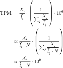
Transcripts per million (TPM) is a measurement of the proportion of transcripts in your pool of RNA.

Since we are interested in taking the length into consideration, a natural measurement is the rate, counts per base (). As you might immediately notice, this number is also dependent on the total number of fragments sequenced. To adjust for this, simply divide by the sum of all rates and this gives the proportion of transcripts in your sample. After you compute that, you simply scale by one million because the proportion is often very small and a pain to deal with. In math:

.

TPM has a very nice interpretation when you’re looking at transcript abundances. As the name suggests, the interpretation is that if you were to sequence one million full length transcripts, TPM is the number of transcripts you would have seen of type , given the abundances of the other transcripts in your sample. The last “given” part is important. The denominator is going to be different between experiments, and thus is also sample dependent which is why you cannot directly compare TPM between samples. While this is true, TPM is probably the most stable unit across experiments, though you still shouldn’t compare it across experiments.

I’m fairly certain TPM is attributed to Bo Li et. al. in the original RSEM paper.

RPKM/FPKM

Reads per kilobase of exon per million reads mapped (RPKM), or the more generic FPKM (substitute reads with fragments) are essentially the same thing. Contrary to some misconceptions, FPKM is not 2 * RPKM if you have paired-end reads. FPKM == RPKM if you have single-end reads, and saying RPKM when you have paired-end reads is just weird, so don’t do it :).

A few years ago when the Mortazavi et. al. paper came out and introduced RPKM, I remember many people referring to the method which they used to compute expression (termed the “rescue method”) as RPKM. This also happened with the Cufflinks method. People would say things like, “We used the RPKM method to compute expression” when they meant to say they used the rescue method or Cufflinks method. I’m happy to report that I haven’t heard this as much recently, but I still hear it every now and then. Therefore, let’s clear one thing up: FPKM is NOT a method, it is simply a unit of expression.

FPKM takes the same rate we discussed in the TPM section and instead of dividing it by the sum of rates, divides it by the total number of reads sequenced () and multiplies by a big number (). In math:

.

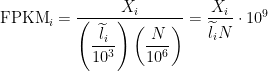
The interpretation of FPKM is as follows: if you were to sequence this pool of RNA again, you expect to see fragments for each thousand bases in the feature for every fragments you’ve sequenced. It’s basically just the rate of fragments per base multiplied by a big number (proportional to the number of fragments you sequenced) to make it more convenient.

Relationship between TPM and FPKM

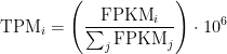
The relationship between TPM and FPKM is derived by Lior Pachter in a review of transcript quantification methods () in equations 10 – 13. I’ll recite it here:

.

If you have FPKM, you can easily compute TPM:

.

Wagner et. al. discuss some of the benefits of TPM over FPKM here and advocate the use of TPM.

---

I hope this clears up some confusion or helps you see the relationship between these units. In the near future I plan to write about how to use sequencing depth normalization with these different units so you can compare several samples to each other.

---

R code

I’ve included some R code below for computing effective counts, TPM, and FPKM. I’m sure a few of those logs aren’t necessary, but I don’t think they’ll hurt :).

countToTpm <- function(counts, effLen)
{
    rate <- log(counts) - log(effLen)
    denom <- log(sum(exp(rate)))
    exp(rate - denom + log(1e6))
}

countToFpkm <- function(counts, effLen)
{
    N <- sum(counts)
    exp( log(counts) + log(1e9) - log(effLen) - log(N) )
}

fpkmToTpm <- function(fpkm)
{
    exp(log(fpkm) - log(sum(fpkm)) + log(1e6))
}

countToEffCounts <- function(counts, len, effLen)
{
    counts * (len / effLen)
}

################################################################################
# An example
################################################################################
cnts <- c(4250, 3300, 200, 1750, 50, 0)
lens <- c(900, 1020, 2000, 770, 3000, 1777)
countDf <- data.frame(count = cnts, length = lens)

# assume a mean(FLD) = 203.7
countDf$effLength <- countDf$length - 203.7 + 1
countDf$tpm <- with(countDf, countToTpm(count, effLength))
countDf$fpkm <- with(countDf, countToFpkm(count, effLength))
with(countDf, all.equal(tpm, fpkmToTpm(fpkm)))
countDf$effCounts <- with(countDf, countToEffCounts(count, length, effLength))

Written by haroldpimentel Posted in Computational biology, Statistics